
How do computers simulate coastlines?
Why are there waves in the ocean, and how can they be modeled using a computer and equations? An article by Maria Kazakova, associate professor at LAMA (Chambéry)

Why are there waves in the ocean?
Waves are among the most fascinating phenomena of motion in the natural world. They can be gentle, almost hypnotic, or sudden and devastating, capable of reshaping entire coastlines in a matter of minutes. For centuries, humans have gazed at the sea and wondered about the movements that animate its surface. At first glance, waves may seem like nothing more than a simple back-and-forth motion of the water, but they are actually the result of complex physical processes.
Most ocean waves are generated by the wind. As air moves across the sea’s surface, it transfers some of its energy to the water, first creating tiny ripples, then larger waves that can travel enormous distances. Some waves generated in storm-tossed ocean regions can continue to propagate long after the wind that created them has died down. Yet wind is just one of many forces capable of setting water in motion. Waves can also be triggered by changes in atmospheric pressure, underwater landslides, volcanic eruptions, or earthquakes beneath the seafloor. The most spectacular example is the tsunami: out at sea, such a wave can go almost unnoticed, standing only a few dozen centimeters high, yet stretching over an immense wavelength. But as it approaches the coast and the water becomes shallower, its speed decreases, its shape changes, and its height can reach that of a destructive wall of water. A phenomenon that is nearly invisible offshore can thus become catastrophic upon reaching the shoreline.
As waves move from deep water toward the shore, they begin to transform. Their speed depends on depth, their crests may curve due to the underwater topography, and their amplitude may increase in a process called “shoaling.” Eventually, a wave can become too steep to remain stable and break, releasing its energy in the form of turbulence, spray, and foam. This familiar coastal spectacle, so common in everyday life, is in fact the end result of a delicate balance between gravity, inertia, depth, and energy dissipation.
| Extreme wave heights can be extraordinary | In 1958 in Lituya Bay, Alaska, a landslide triggered by an earthquake caused a megatsunami: a giant wave 60 meters high, traces of which were observed up to an altitude of 525 meters. This makes it one of the most extreme wave phenomena ever recorded. |
| Internal waves can be much stronger than surface waves | Not all waves are visible at the surface. The ocean also harbors hidden waves that propagate at depth, along layers of water with different densities and salinity levels. These waves can reach amplitudes of over 100 meters, and in some regions, even over 200 meters, while remaining virtually invisible from the surface. |
| Tsunamis can travel across the oceans at remarkable speeds | In the open ocean, tsunami waves can travel at speeds of several hundred kilometers per hour—typically around 800 km/h and, according to some sources, up to about 1,000 km/h—allowing them to cross ocean basins in just a few hours before slowing down in shallow coastal waters. |
Mathematical Models
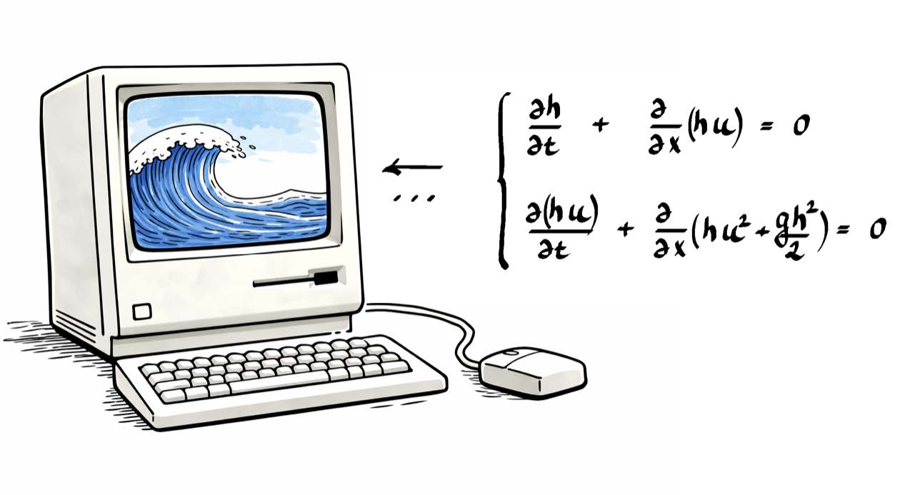
Studying waves involves working at the intersection of physics, mathematical modeling, and numerical computation. Wave motion can be described by mathematical models formulated as systems of differential equations, such as the well-known shallow-water equations (Barré-de-Saint-Venant equations). In collaboration with physicists, mathematicians are developing increasingly complex models capable of better representing the complexity of real-world wave behavior, including breaking waves. In these models, the equations describe the evolution over time of quantities such as water height or velocity at each point in space.
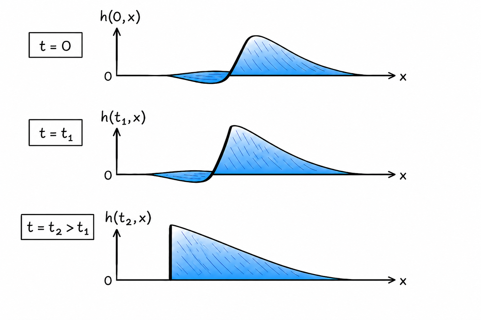
Figure 2 illustrates the evolution of a water-depth profile obtained using a highly simplified equation known as the Burgers equation. Although not very realistic, it is still sufficiently detailed to highlight important wave phenomena such as propagation, surface stiffening, and the formation of very distinct fronts. Due to its abrupt profile (referred to here as a discontinuity), this type of solution is called a “shock wave.” Such solutions have proven their relevance in modeling wave breaking, which is an otherwise complex subject. What makes this example particularly interesting is that, precisely because of this discontinuity, the equation alone does not determine a unique solution. In other words, several mathematically valid solutions may exist, but only one corresponds to the physical behavior observed in nature.
Once the equations are established, computers become essential tools for making predictions and understanding how the model behaves in practice.
What instructions do we need to give computers so they can model waves?
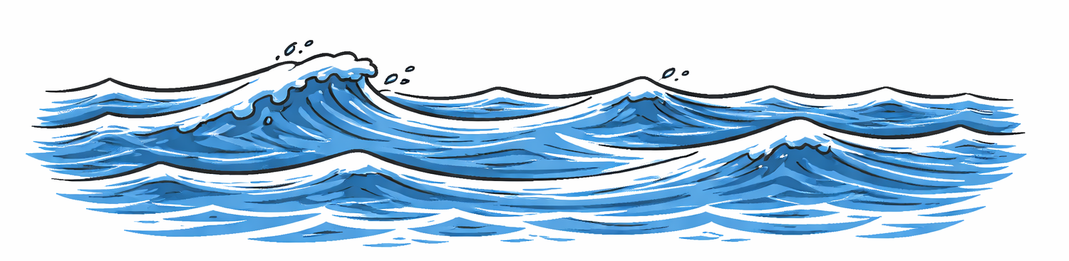
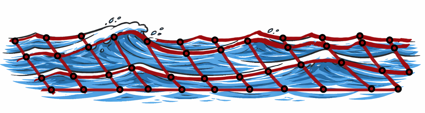
In mathematics, wave equations are formulated in a continuous space and time. Computers, on the other hand, are discrete machines: they do not handle continuous objects, but rather finite sets of numbers. This gap is bridged by what is known as the discretization of the domain, one of the fundamental principles of numerical analysis. Rather than describing the wave at every point on the water’s surface, we do so only for a finite set of positions, called nodes. The illustration below (Figure 3) illustrates this principle: although the water surface is physically continuous, much like a fabric, we represent it using a grid consisting of a finite number of nodes placed on this continuous surface. Time is discretized in a similar manner.
At this stage, the mathematician’s task is to develop a method, known as a “numerical scheme,” that transforms the equations into an algorithm that can be implemented on a computer, and that involves updating the values associated with the nodes at each time step. Such an algorithm must satisfy essential properties, notably stability and convergence toward the correct solution. Put simply, stability ensures that the calculation proceeds correctly—for example, without developing unwanted oscillations—while convergence ensures that the numerical approximation improves as the grid is refined, that is, when there are more nodes and they are closer together. This provides a more detailed description of the wave, at the cost of increased computational time and resources.
A high-quality numerical scheme must also respect fundamental physical properties. For example, the water depth must always remain positive, and the system’s energy must evolve realistically. In particular, it must not increase artificially during the calculation: in real-world flows, processes such as friction or wave breaking tend to dissipate energy rather than create it. If these principles are not followed, the solution cannot correspond to a real physical situation.
The Importance of Choices Made When Developing a Numerical Algorithm
There are many numerical schemes for a single equation, and they do not necessarily produce the same results. When the solution remains smooth, these differences may be minimal. However, in the presence of sharp fronts (discontinuities), the choice of scheme becomes critical: some methods reproduce the correct physical behavior, while others may lead to inaccurate or even non-physical solutions. More specifically, when solving the equation numerically, one must decide how the wave propagates through the grid—in other words, how information is transmitted from one grid point to its neighbors. Several options are available: some schemes smooth out the discontinuity, while others, on the contrary, attempt to follow it more precisely. These choices determine how the wave is reconstructed between the grid points and can lead to very different results.
Here we wish to present a simple example of the discretization of the Burgers equation, which, at first glance, may not seem closely related to waves. But it allows us to show, very clearly, that the result of a simulation depends not only on the equation itself, but also on the numerical method used to approximate it.
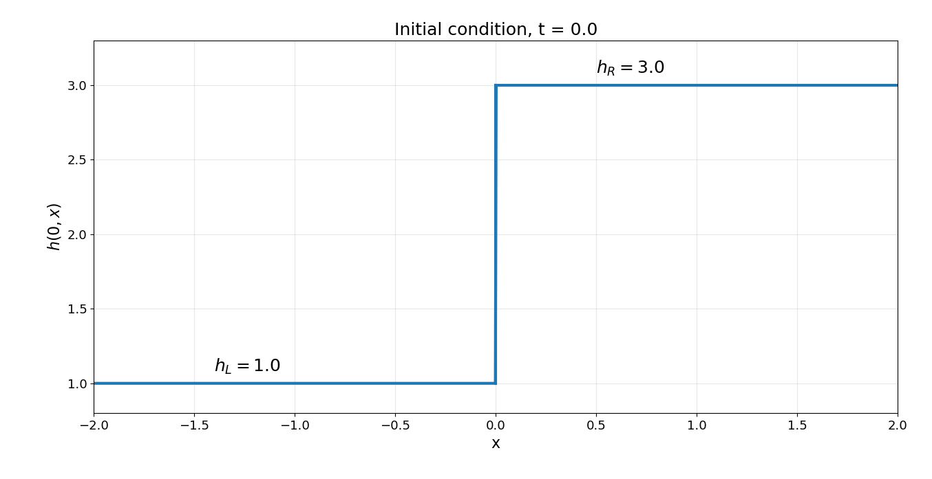
Let’s consider a simple situation where the water has two different levels at time 0. Imagine a column of water next to an area where the water level is lower. In mathematical terms, this is expressed by the following initial condition:
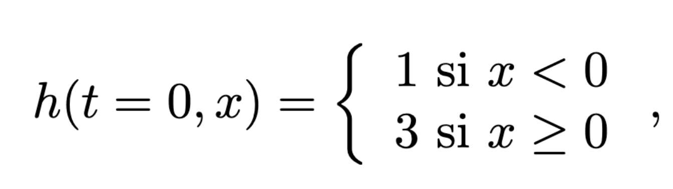
as shown below:
Here (Figure 5), we compare the results of two numerical schemes that approximate the solutions to the Burgers equation. Each scheme produces a mathematically valid solution to the equation, but only one of them captures the expected wave dynamics. It is shown in orange in Figure 6. This solution is correctly reproduced by the scheme shown in the figure on the right.
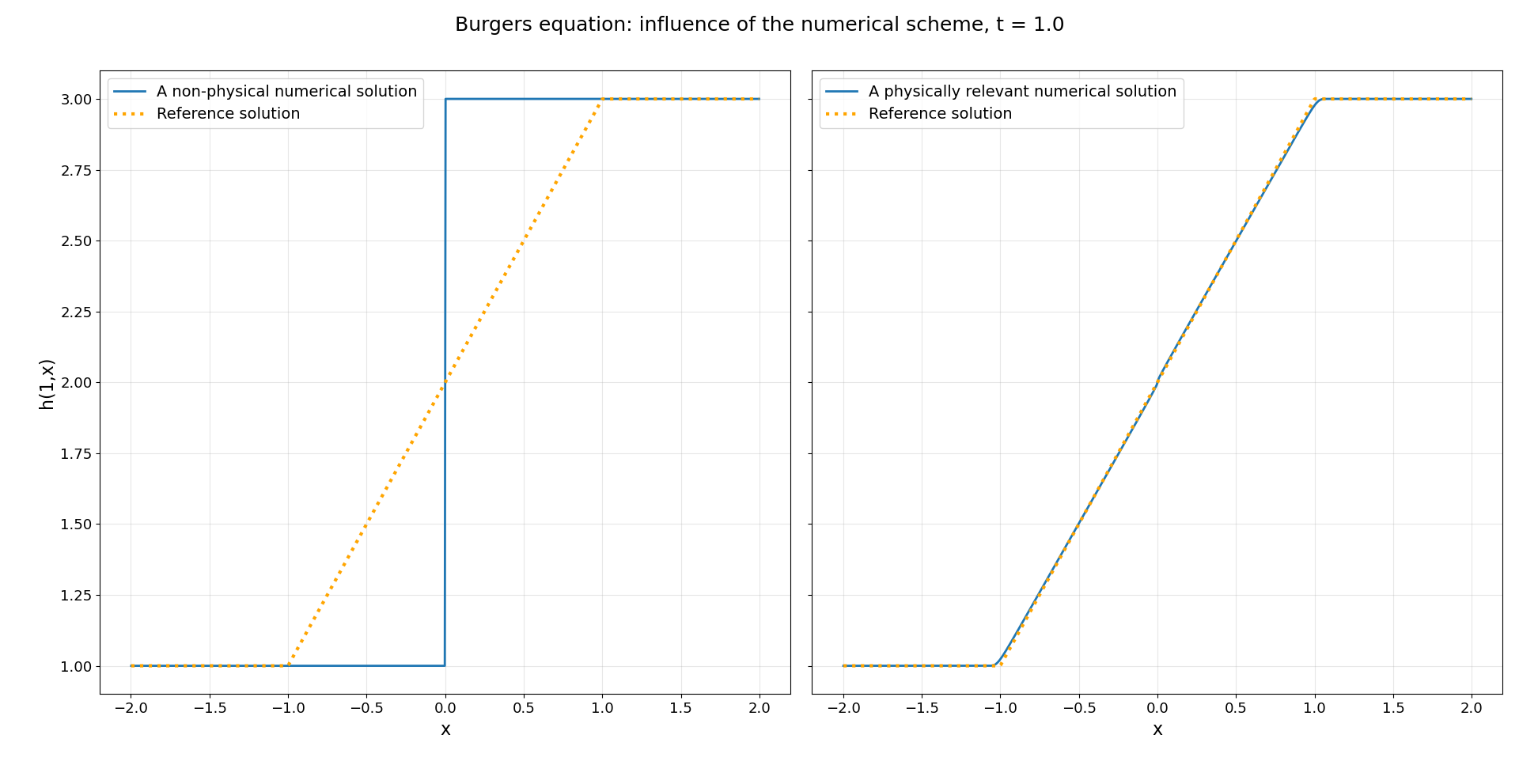
What makes the result on the left amusing is that this non-physical solution seems to suggest that, if a column of water is initially at rest, it will simply remain frozen in space instead of collapsing under the force of gravity.

Thus, even though this example does not directly describe real coastal waves, it teaches us an important lesson about wave modeling in general: before relying on a simulation, we must ensure that the numerical method is capable of selecting the correct physical solution, which itself is determined by a detailed theoretical analysis of the equations. Here we see that the interaction between mathematics, physics, and mechanics is essential.