
Mathematics for Mapping Major Ocean Currents
How can we create an accurate map of major ocean currents? How can we predict their behavior? An article by Anne-Laure Dalibard, a faculty researcher at the Jacques-Louis Lions Laboratory.
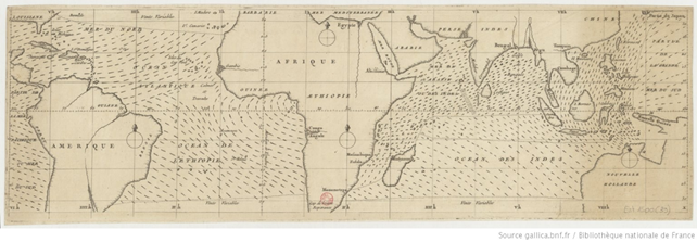
How can we create an accurate map of major ocean currents? The first answer that comes to mind is undoubtedly to observe them and record the speed of the currents at each point. This is, in fact, how old nautical charts were created, and for centuries they played a crucial role in navigation.
But observing current speeds at any point on the globe is no easy task, even with today’s tools: in particular, satellite observations are mainly used to measure disturbances at sea level.
Using our knowledge of the physical principles that govern the ocean, we will see how sea level is related to current speed through geostrophic equilibrium. We will also explain how we can predict future changes in these speeds and understand certain important properties of ocean circulation, such as the intensification of currents along the western edges of the oceans (that is, off the eastern coasts of the continents!).
Geostrophic Equilibrium
Let’s start with an overview of the forces acting on ocean currents. The ocean is subject to several external forces: gravity, the gravitational pull of the Moon and the Sun (which create the tides), and interactions with the atmosphere, coastlines, and the seafloor… In addition to these, there are internal forces, such as pressure (well known to scuba divers!), as well as the Coriolis force, which is caused by the Earth’s rotation. The Coriolis force always acts perpendicular to the direction of motion, deflecting it to the right in the Northern Hemisphere and to the left in the Southern Hemisphere. Its effect is visible on the map below: on a global scale, ocean currents organize themselves into “gyres”—that is, gigantic whirlpools several thousand kilometers in diameter.
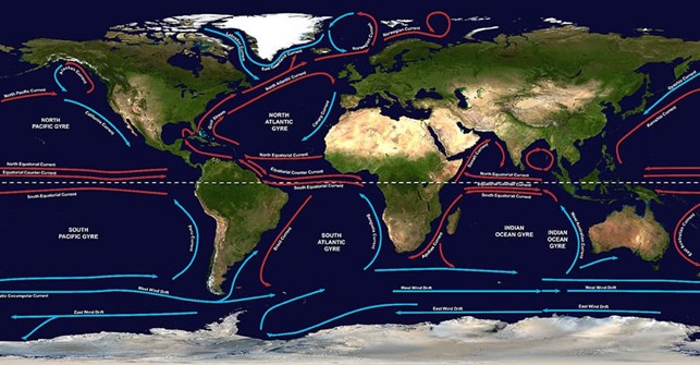
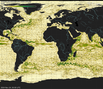
On large horizontal scales, the Coriolis force almost exactly balances the horizontal component of pressure forces. This is referred to as “geostrophic equilibrium” (from the Ancient Greek “gê,” meaning Earth, and “strophê,” meaning rotation). However, horizontal pressure fluctuations are proportional to sea-level changes, which can be observed by satellite. This is how satellite observations make it possible to map so-called “geostrophic” currents, as shown in the following figure.
The Importance of Scale Models
Observations provide information only on current velocities at a given moment: to predict their future behavior, we must turn to physical models. These models govern the dynamics of currents through a complex system of differential equations. This system is an “extended” version of the well-known Navier–Stokes equations in fluid mechanics and thus inherits all the associated mathematical difficulties. It is therefore impossible to have a formula that explicitly calculates current velocity.
To describe currents despite these difficulties, scientists have various tools at their disposal, which can, of course, be combined. First, the system can be simplified by comparing the relative importance of the different terms and neglecting certain effects in favor of others: this is precisely what we did earlier when describing geostrophic equilibrium. This leads to “reduced” models, which are easier to analyze, even if they may be less accurate in representing reality. We can also calculate an approximate value for the speed of the currents—or other quantities of interest—using a computer, as described in the article “How Do Computers Simulate the Coastline?.” However, this requires considerable computing power and time, due to the immense size of the oceans. Finally, a qualitative description of the currents is sometimes sufficient. In other words, we do not necessarily seek to know the precise value of their speed, but only certain properties: Is the current flowing north or south? In which region is it strongest? This is what we will do in the last part of this article.
Let’s now return to geostrophic equilibrium. As we saw earlier, predicting the evolution of geostrophic currents amounts to predicting the evolution of pressure. We must therefore write an equation that governs the latter!
Fortunately, a well-known “simplified model” in oceanography does precisely that, linking the temporal and spatial variations in pressure. By then cleverly applying geostrophic equilibrium, we can deduce the geostrophic velocity of the currents. This model, known as “quasi-geostrophic,” is considerably simpler to analyze than the complete system, while still accurately predicting many oceanographic phenomena.
Western Edge Currents
Among the notable predictions of the quasi-geostrophic model, let us now turn our attention to the western edge currents: in a relatively narrow zone (on the order of a few tens of kilometers) near the coasts to the west of the ocean basins, the currents flow at very high speeds and are tangent to the edge; to conform to the direction of rotation of the gyres described above, this velocity is directed northward in the Northern Hemisphere and southward in the Southern Hemisphere. These currents play a crucial role in global dynamics, as they transport heat from the tropics toward the poles. Several well-known currents, such as the Gulf Stream along the U.S. coast, the Aiguilles Current in the Indian Ocean, and the Kuroshio off the coast of Japan, are western boundary currents.
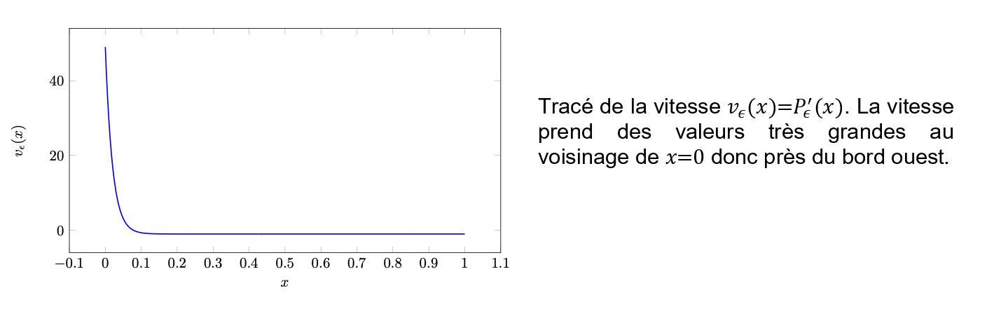
Mathematically, these currents can be described using the boundary layer formalism: a certain quantity (in this case, pressure) varies significantly within a restricted zone near the edge of the studied domain. In the quasi-geostrophic model, the tangential velocity at the boundary is the derivative of the pressure. If this pressure varies greatly, the velocity is therefore very high.
Solution to the differential equation
By further manipulating and simplifying the equations of the quasi-geostrophic model, we can derive a very simple differential equation, the solution to which is shown in the following figure:
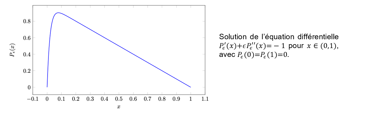
Here, in a highly idealized case (sometimes referred to as a “toy model”), we plot the variations in pressure \(P_ϵ\) as a function of longitude \(x\): corresponds to the western end of the basin, and
  to its eastern end. The number
  is a small parameter, set equal to 0.02 in the figure above
We see that the function \(P_ϵ\) varies from zero to values close to 1 over an interval of length comparable to \(ϵ\) at the western end. Its derivative, the velocity, is therefore of the order of \(1⁄ϵ\) over this interval and consequently very intense: this is precisely the mechanism behind the formation of western boundary currents; since the velocity is positive here, it is a simplified analogy, for example, of the Gulf Stream.
The reality is, of course, quite different from this highly simplified model. First of all, as is obvious, ocean basins are three-dimensional: variations in pressure along the other dimensions (latitude, depth) must therefore be taken into account, and the geometry of the coastlines and the seafloor can come into play and significantly complicate the analysis! Furthermore, the simplified model above overlooks many effects that can play an important role.
Faced with this complexity, scientists from various disciplines (oceanography, mathematics, physics, etc.) are joining forces to improve our understanding of ocean currents. For example, mathematically understanding the behavior of simplified models like the one presented above makes it possible to modify certain numerical codes in climate models and better represent specific phenomena. As a result, several research teams are currently working to improve our understanding of the Gulf Stream’s separation off the coast of Florida: near Cape Hatteras, the Gulf Stream veers eastward and separates from the coast, before becoming destabilized and generating numerous highly energetic eddies. The mechanisms at work in this separation phenomenon remain largely misunderstood, despite their crucial importance in describing Earth’s climate, and represent a fascinating scientific challenge!